
Max Simmonds
M.Eng (Hons) First Class
Software engineer at Starship Technologies and co-founder of Purple Parrot. Previously at CERN and ESA. MEng (Hons, 1st) from the University of Plymouth. Based in Tallinn, Estonia.
Project Status
FFT and Fourier — Intuition, Derivation, and the Link to Fortescue
This builds from first principles: eigenvalues, eigenfunctions, what a frequency is, why sine waves are special, how the DFT detects them, why the FFT is fast, and how Fortescue’s symmetrical components are just a 3-point DFT applied to motor phases.
Contents
- Eigenvalues and eigenvectors
- Eigenfunctions — the same idea for functions
- What is a frequency, really?
- Fourier’s claim
- Euler’s formula — the rotating arrow
- The DFT — detecting a frequency by correlation
- The DFT matrix — it’s just matrix multiplication
- The FFT — why it’s fast
- Fortescue = 3-point DFT
- The unified picture
1. Eigenvalues and eigenvectors
The problem eigenvectors solve
A matrix transforms vectors — it rotates them, stretches them, shears them. In general, if you multiply a vector v by a matrix A, the output Av points in a completely different direction.
But for every matrix there exist a few special directions where this isn’t true. Vectors pointing in these directions get stretched or shrunk, but never rotated. These are the eigenvectors.
The equation:
A·v = λ·v
Says: applying matrix A to vector v gives back the same vector v, just scaled by the number λ. That number is the eigenvalue — it tells you how much the eigenvector gets stretched (λ > 1), shrunk (0 < λ < 1), flipped (λ < 0), or unchanged (λ = 1).
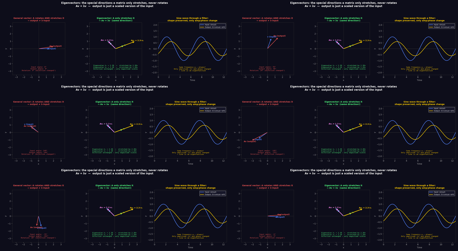
Left: a general vector gets rotated AND stretched by matrix A — direction changes. Middle: eigenvectors v₁ and v₂ only get stretched — direction is preserved, Av = λv exactly. Right: a sine wave through a filter — same frequency out, only amplitude and phase change. Sine waves are eigenfunctions.
Finding eigenvalues
Rearrange Av = λv as (A - λI)v = 0. For this to have a non-trivial solution (v ≠ 0), the matrix (A - λI) must be singular — its determinant must be zero:
det(A - λI) = 0
This is the characteristic equation. Solving it gives you the eigenvalues λ. Plug each λ back into (A - λI)v = 0 to find the corresponding eigenvector.
Example — 2×2 matrix
A = [3  1]
    [0  2]

det(A - λI) = det([3-λ   1 ]) = (3-λ)(2-λ) - 0 = 0
                  [0    2-λ])

→ λ₁ = 3,  λ₂ = 2
For λ₁ = 3: (A - 3I)v = 0 → v₁ = [1, 0] (x-axis, stretched 3×)
For λ₂ = 2: (A - 2I)v = 0 → v₂ = [1, -1] (diagonal, stretched 2×)
Why eigenvalues matter
Eigenvectors are the natural coordinate system of a matrix. If you express everything in eigenvector coordinates, the matrix becomes diagonal — each component just scales independently, no mixing. This makes computation trivial.
This is why eigendecomposition is everywhere: PCA (data science), vibration modes (mechanical engineering), quantum states (physics), and — as we’re about to see — frequency analysis.
2. Eigenfunctions — the same idea for functions
Operators, not matrices
In signal processing and physics, you often apply operators to functions rather than matrices to vectors. An operator takes a function in and spits a function out. Examples:
- Differentiation:
L[f] = df/dt - Integration:
L[f] = ∫f dt - Convolution:
L[f] = f * h(filtering)
An eigenfunction of operator L is a function f where:
L[f] = λ·f
The operator produces the same function back, just scaled by λ. Exact same idea as eigenvectors, just for functions instead of vectors.
Sine waves as eigenfunctions of differentiation
Take the derivative operator d/dt and apply it to e^(jωt):
d/dt [e^(jωt)] = jω · e^(jωt)
The output is the same function e^(jωt), scaled by jω. So e^(jωt) is an eigenfunction of d/dt with eigenvalue jω.
Since e^(jωt) = cos(ωt) + j·sin(ωt), this means sine and cosine are eigenfunctions of differentiation.
Sine waves as eigenfunctions of any LTI system
An LTI system (Linear Time-Invariant) is any system where:
- Scaling the input scales the output (linear)
- Shifting the input shifts the output in time (time-invariant)
Motor windings, filters, amplifiers, transmission lines — all LTI.
Proof that sine waves are eigenfunctions of any LTI system:
An LTI system is fully described by its impulse response h(t). Its output for any input x(t) is convolution:
y(t) = (h * x)(t) = ∫ h(τ) · x(t-τ) dτ
Put in x(t) = e^(jωt):
y(t) = ∫ h(τ) · e^(jω(t-τ)) dτ
     = e^(jωt) · ∫ h(τ) · e^(-jωτ) dτ
     = e^(jωt) · H(jω)
Where H(jω) = ∫ h(τ) e^(-jωτ) dτ is just a complex number — the frequency response at frequency ω.
So:
y(t) = H(jω) · e^(jωt) = λ · x(t)
| The output is the same frequency, scaled by complex number H(jω). Eigenfunction confirmed. The eigenvalue is H(jω) — it tells you how much the system amplifies ( | H | ) and phase-shifts (∠H) at that frequency. |
Why this makes Fourier transforms work
Because sine waves are eigenfunctions of LTI systems, they’re the natural basis to analyse them in. If you decompose your input into sine waves (Fourier transform), each component passes through the system independently — scaled by its eigenvalue H(jω). The output is just the sum of scaled components.
This is why:
- You can design a filter by shaping H(jω) in the frequency domain
- Motor control is done in the dq frame (which isolates the positive-sequence eigenfunction)
- FOC gives clean torque control — you’re working directly with the eigenfunction of the motor system
3. What is a frequency, really?
A frequency is just a sine wave repeating at a particular rate. That’s it.
f = 1 Hz  →  one full cycle per second
f = 3 Hz  →  three full cycles per second
What makes sine waves special is that they are eigenfunctions of linear systems — if you put a sine wave into any linear system (a filter, a motor winding, an amplifier), the output is also a sine wave at the same frequency. Only the amplitude and phase can change, never the frequency.
This is why frequency analysis is so powerful: it’s the natural language of linear systems.
4. Fourier’s claim
Jean-Baptiste Fourier (1822) made a claim that seemed absurd at the time:
Any periodic signal, no matter how complicated, can be written as a sum of sine waves.
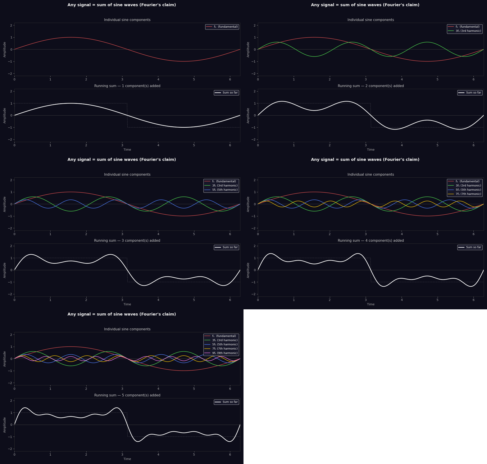
A square wave being built up from odd harmonics: f, 3f, 5f, 7f… Each frame adds one more sine wave. More components = sharper corners.
The coefficients (how much of each sine wave) are what the Fourier transform computes. The transform doesn’t change the signal — it just re-describes it in frequency language instead of time language.
Same information, different perspective. Like describing a location as (x, y, z) vs (r, θ, φ) — same point, different coordinates.
5. Euler’s formula — the rotating arrow
(Based on 3Blue1Brown’s “What is Euler’s formula actually saying?” — Lockdown Live Math ep. 4, and “Euler’s formula via group theory”)
Before the DFT, you need to understand Euler’s formula:
e^(jθ) = cos(θ) + j·sin(θ)
This connects the exponential function to rotation. A complex exponential is just an arrow rotating in the complex plane.
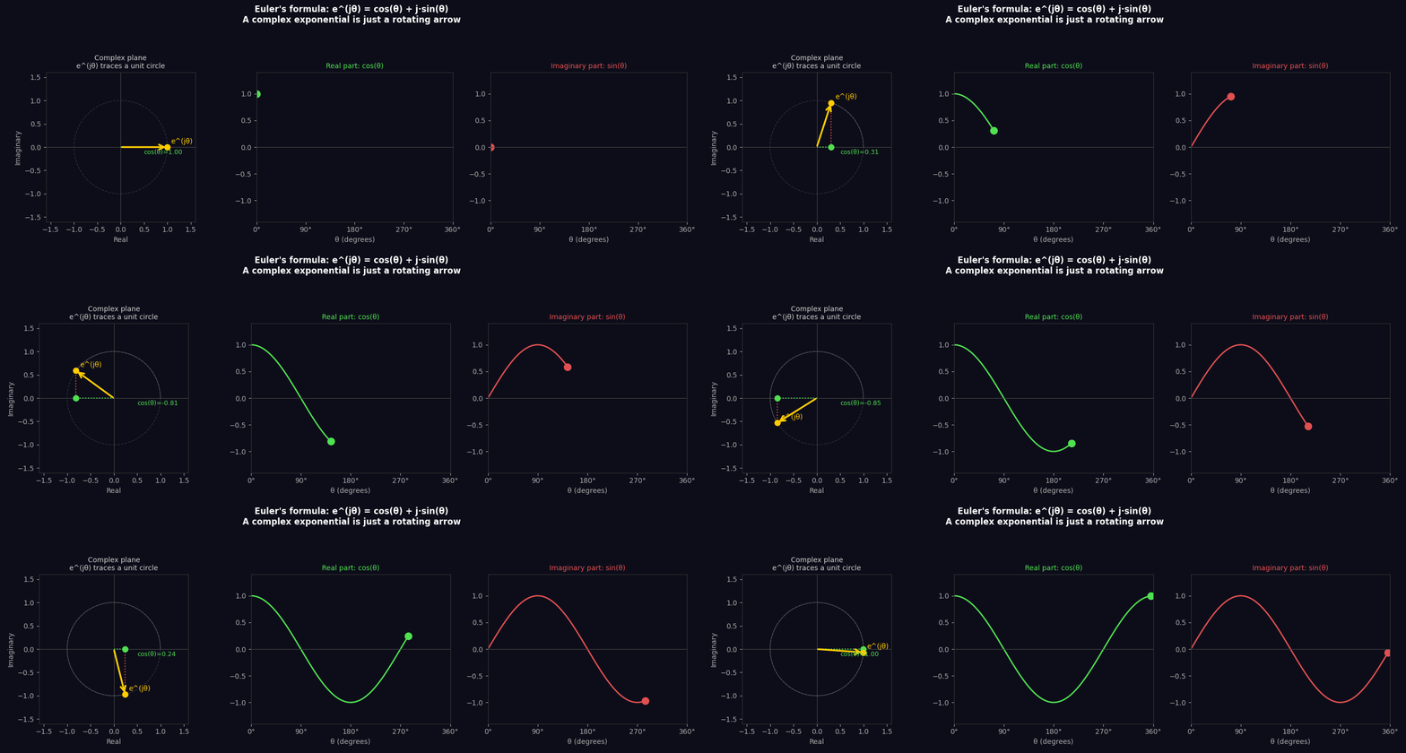
Left: the phasor e^(jθ) rotating on the unit circle. Middle: its real part traces a cosine. Right: its imaginary part traces a sine. They’re the same thing viewed from different angles.
The problem with the notation
e^2 makes sense — multiply e by itself twice. e^(jπ)? You can’t multiply something by itself an imaginary number of times. The standard notation seems broken.
The fix: stop thinking about what exponentiation is and think about what it does.
The group theory view — two worlds of number actions
Numbers can act on the world in two fundamentally different ways:
World 1 — Sliding (additive group) Numbers as movements along a line. 3 means “slide right by 3”. -2 means “slide left by 2”. Combining two slides adds the distances. On the complex plane, imaginary numbers slide vertically — j means “slide up by 1”.
World 2 — Stretching and rotating (multiplicative group) Numbers as transformations of the plane. 3 means “stretch by factor 3”. j means “rotate 90°”. Combining two transformations multiplies them — rotating 90° twice gives 180°.
These are two completely separate worlds with different arithmetic. But there’s a bridge.
The bridge — exponentials as homomorphisms
A homomorphism is a function that converts the arithmetic of one world into the arithmetic of another while preserving structure.
Exponentials do exactly this:
e^(a+b) = e^a · e^b
Adding in the sliding world = multiplying in the stretching/rotating world. The exponential function translates between them. This is why it appears everywhere in physics — anything involving growth, oscillation, or rotation has addition and multiplication secretly connected underneath.
Specifically:
- Real inputs (horizontal slides) → stretching/shrinking outputs
- Imaginary inputs (vertical slides) → pure rotation outputs
A vertical slide of θ units maps to a rotation of θ radians. That’s what e^(jθ) means — not a strange power, but a translation of the sliding action jθ into the rotating action “rotate by θ”.
Why e specifically — the unit speed argument
For a general base b, a vertical slide of 1 unit maps to a rotation of ln(b) radians. Different bases rotate at different speeds.
e is the unique base where a vertical slide of 1 unit maps to exactly 1 radian of rotation — unit speed, no scaling factor.
Base 2:   vertical slide of 1  →  rotation of ln(2) ≈ 0.693 rad
Base 3:   vertical slide of 1  →  rotation of ln(3) ≈ 1.099 rad
Base e:   vertical slide of 1  →  rotation of ln(e) = 1.000 rad  ✓
Any other base introduces a constant everywhere. e is the one where the map is “natural” — identity speed between the two worlds.
What e^(jπ) = -1 actually says
Start at position 1 on the complex plane (the point (1, 0)).
Apply the action e^(jπ): a vertical slide of π units, translated into a rotation of π radians.
Rotating 1 by π radians (180°) lands you at -1.
e^(jπ) = -1 means: "rotate 180° and you end up at the opposite point"
No magic. Just geometry. The famous formula is just saying: half a turn takes you to the other side.
What this means for motors and FOC
Every rotating phasor in this entire document is e^(jωt) — the sliding action jωt (imaginary, so vertical, so a rotation) translated into a multiplicative rotation at rate ω.
The Park transform × e^(-jθ) means: apply the action of rotating by -θ. Undo the rotor’s rotation. The minus sign isn’t arbitrary — it’s the inverse in the multiplicative group, which corresponds to a negative slide in the additive group.
Fortescue’s a = e^(j2π/3) is a vertical slide of 2π/3, translated to a rotation of exactly 120°.
The whole machinery — Clarke, Park, Fortescue, DFT — is the exponential homomorphism being used to move between the additive world (angles that add) and the multiplicative world (rotations that compose).
Why j (imaginary unit)?
j = √(-1). Multiplying by j rotates a complex number by 90°:
1   × j = j        (0° → 90°)
j   × j = -1       (90° → 180°)
-1  × j = -j       (180° → 270°)
-j  × j = 1        (270° → 360° = 0°)
Repeated multiplication by j is rotation. The exponential e^(jθ) generalises this to any angle — it’s the smooth version of repeatedly multiplying by j.
Negative frequency
e^(-jθ) rotates in the opposite direction — clockwise. This is negative frequency. It’s not mysterious — it’s the inverse rotation action in the multiplicative group, which the homomorphism maps to a negative slide in the additive group.
When you multiply a signal by e^(-jωt) you are applying the inverse of rotation ω — if the signal contains a component rotating at ω, the two rotations cancel to zero. It becomes DC.
This is the entire mechanism of the Park transform and the DFT.
6. The DFT — detecting a frequency by correlation
The problem
You have N samples of a signal x[0], x[1], ..., x[N-1]. You want to know: how much of frequency k is in this signal?
The answer — correlation
Multiply each sample by the complex conjugate of the frequency-k template, then sum:
X[k] = Σ x[n] · e^(-j2πkn/N) for n = 0, 1, ..., N-1
This is the Discrete Fourier Transform (DFT).
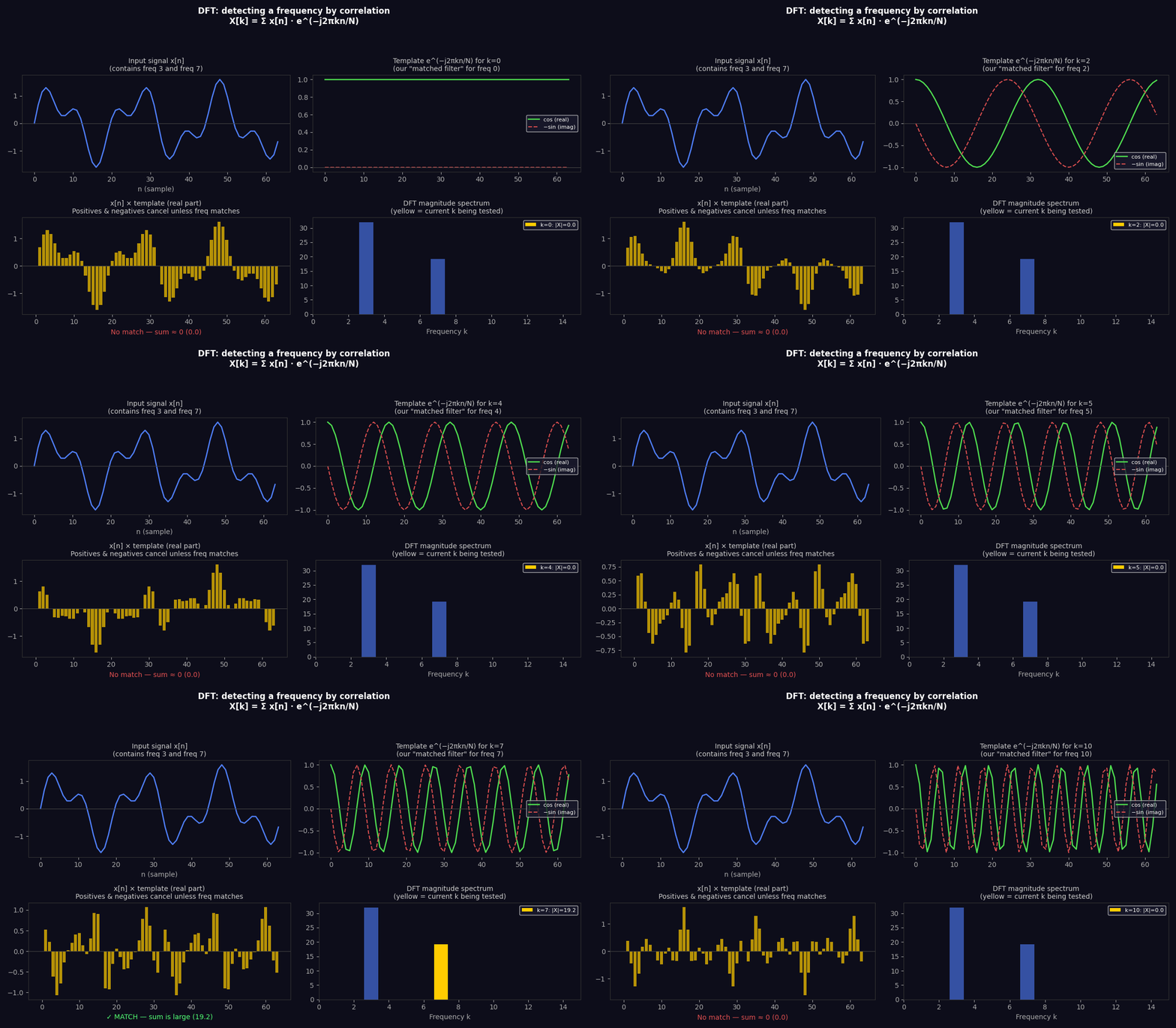
The yellow bar sweeps through frequency bins k=0 to 10. When k matches a frequency in the signal (k=3 and k=7), the products all align and sum to a large value. Everywhere else they cancel.
Why does it work?
For each sample x[n], you multiply by e^(-j2πkn/N). This rotates the sample backwards by angle 2πkn/N — exactly the angle that a frequency-k component would have accumulated by sample n.
If the signal contains frequency k:
- All rotated samples point the same direction
- They add constructively
|X[k]|is large
If the signal does not contain frequency k:
- Rotated samples point in random directions
- They cancel
|X[k]|≈ 0
This is why the DFT is called a matched filter — the template e^(-j2πkn/N) is shaped exactly like frequency k. It resonates with its own frequency and rejects everything else.
The output
X[k] is a complex number. Its magnitude |X[k]| tells you how much of frequency k is present. Its angle ∠X[k] tells you the phase.
7. The DFT matrix — it’s just matrix multiplication
Write all N DFT outputs at once:
X = W · x
Where W is the N×N DFT matrix:
        [  1      1        1        1     ...  ]
        [  1      W^1      W^2      W^3   ...  ]
W  =    [  1      W^2      W^4      W^6   ...  ]
        [  1      W^3      W^6      W^9   ...  ]
        [  ...                              ...  ]

where W = e^(-j2π/N)   (the N-th root of unity)
Entry W[k,n] = e^(-j2πkn/N) — rotating the n-th sample back by k steps.
The DFT matrix is a unitary matrix — its inverse is just its conjugate transpose scaled by 1/N:
W^(-1) = (1/N) · W* (complex conjugate)
This means the DFT is perfectly reversible. No information lost — just a change of basis.
The 3×3 case — preview of Fortescue
For N=3:
W = e^(-j2π/3) → W^0=1, W^1=a*, W^2=a²*
Where a = e^(j2π/3) is Fortescue’s rotation operator. The 3-point DFT matrix is:
[X[0]]   [1    1     1  ] [x[0]]
[X[1]] = [1    W     W² ] [x[1]]   × (1/3)
[X[2]]   [1    W²    W⁴ ] [x[2]]
This is exactly the Fortescue transform. The sequences are just DFT frequency bins at N=3.
8. The FFT — why it’s fast
The problem with the DFT
Computing X[k] requires N multiplications. Computing all N outputs requires N² multiplications total.
For N = 1024: 1,048,576 multiplications. For N = 1,000,000: 10¹² multiplications (takes hours).
The DFT is too slow for real-time use.
Cooley-Tukey’s insight (1965)
Split the N-point DFT into two N/2-point DFTs — one for even-indexed samples, one for odd:
X[k] = Σ x[n]·W^(kn)                              (all N samples)
     = Σ x[2m]·W^(2km) + Σ x[2m+1]·W^(k(2m+1))  (split even/odd)
     = Σ x[2m]·(W²)^(km) + W^k · Σ x[2m+1]·(W²)^(km)
     = E[k]  +  W^k · O[k]
Where:
E[k]= N/2-point DFT of even samplesO[k]= N/2-point DFT of odd samplesW^k= twiddle factor (just a rotation)
The butterfly operation
X[k]       = E[k]  +  W^k · O[k]
X[k + N/2] = E[k]  -  W^k · O[k]
Two outputs from two half-size DFTs plus one multiply. This is the butterfly — the basic building block of the FFT.
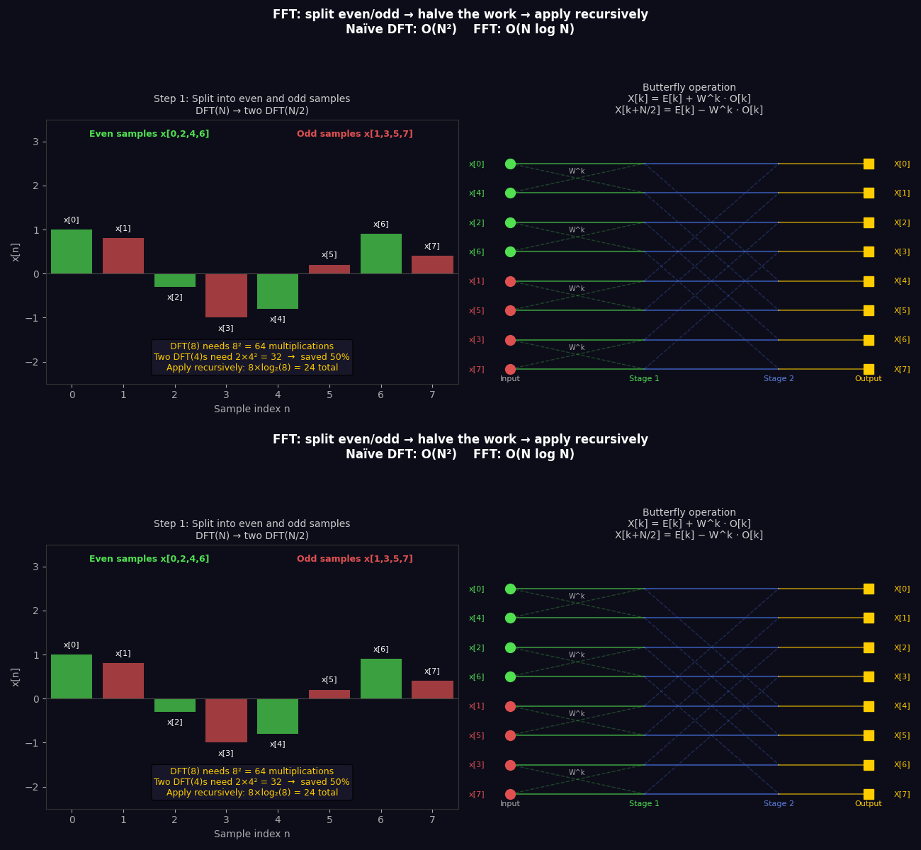
Left: the even/odd split halves the problem. Right: the butterfly diagram showing how each stage combines two half-size DFTs. Three stages for N=8.
The recursion
Apply the split recursively:
DFT(N) → 2 × DFT(N/2)
       → 4 × DFT(N/4)
       → 8 × DFT(N/8)
       → ...
       → N × DFT(1)    (trivial — just the sample itself)
Each level has N multiplications. There are log₂(N) levels.
Total: N·log₂(N) multiplications.
N = 1024:   naive DFT = 1,048,576    FFT = 10,240      (100× faster)
N = 1M:     naive DFT = 10¹²        FFT = 20,000,000  (50,000× faster)
This is why real-time audio, radar, MRI, WiFi, 4G, and motor drives can all use frequency analysis — without the FFT, none of it would be computationally feasible.
Requirement
Cooley-Tukey FFT requires N = 2^m (power of 2). This is why FFT sizes are always 256, 512, 1024, 2048… Zero-padding a signal to the next power of 2 is standard practice.
9. Fortescue = 3-point DFT
Now put it all together.
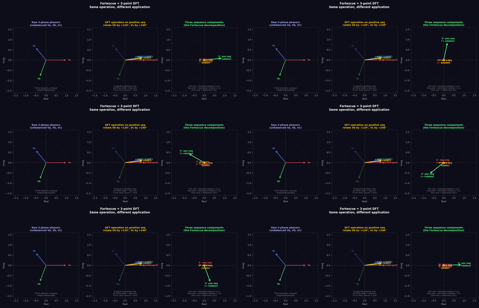
Left: raw unbalanced phasors Va, Vb, Vc. Middle: the DFT operation for positive sequence — rotate Vb by 120°, Vc by 240°, then sum. If the system is positive sequence, all three align → big result. Right: the three sequences animated — positive rotates forward, negative rotates backward, zero is static.
The 3-point DFT explicitly
For N=3 samples (Va, Vb, Vc) and twiddle factor W₃ = e^(-j2π/3):
X[0] = Va + Vb        + Vc             (k=0, DC / zero sequence)
X[1] = Va + W₃·Vb    + W₃²·Vc        (k=1, fundamental forward)
X[2] = Va + W₃²·Vb   + W₃⁴·Vc        (k=2, fundamental backward)
Now note that W₃ = e^(-j2π/3) = a* (complex conjugate of Fortescue’s a).
Rewriting with Fortescue’s a = e^(+j2π/3):
V⁰ = ⅓(Va  + Vb    + Vc  )     ← X[0]/3 = zero sequence
V⁺ = ⅓(Va  + a·Vb  + a²·Vc)   ← X[1]/3 = positive sequence
V⁻ = ⅓(Va  + a²·Vb + a·Vc )   ← X[2]/3 = negative sequence
This is literally the Fortescue transform. The only difference from the standard DFT is the sign convention on the rotation operator — Fortescue defines a as positive rotation (forward), whereas the DFT defines its twiddle factor as negative rotation (backward). They’re the same thing, just looking from opposite directions.
What each bin means physically
| DFT bin k | Frequency | Fortescue name | Physical meaning in motor |
|---|---|---|---|
| 0 | DC | Zero sequence | All phases in phase — fault current |
| 1 | +f | Positive sequence | Forward MMF — useful torque |
| 2 = −1 | −f | Negative sequence | Backward MMF — braking, heat |
Why there are only 3 bins for 3 samples
The DFT of N samples gives you exactly N frequency bins. For N=3 you get 3 bins — DC, +f, and −f. You cannot resolve more than 3 frequencies from 3 samples. This is the Nyquist-Shannon sampling theorem at the most basic level.
For a 3-phase motor, 3 samples (one per phase) is exactly the right number to resolve the three possible symmetrical states. Nature and mathematics align perfectly.
10. The unified picture
Every transform in this chain is doing the same thing:
Change basis to make the signal easier to work with.
The matched filter thread
Every step is a matched filter:
- DFT bin k — matched to frequency k, rejects all others
- Fortescue V⁺ — matched to positive sequence, rejects negative and zero
- Clarke αβ — extracts positive sequence in real coordinates
- Park dq — matched filter + reference frame switch, freezes positive sequence as DC
- PI controller — effectively a matched filter for DC (infinite gain at zero frequency)
The frame switch thread
Every step is also a reference frame change:
- DFT — time domain → frequency domain
- Fortescue — phase domain (abc) → sequence domain (0, +, −)
- Park — stationary frame (αβ) → rotating frame (dq)
- Field weakening — dq frame at ω → dq frame at different operating point
Same idea, different application, different level of abstraction.
Key numbers to remember
DFT:        X[k] = Σ x[n] · e^(-j2πkn/N)
FFT:        O(N log N)  vs  O(N²) for naive DFT
Fortescue:  V⁺ = ⅓(Va + a·Vb + a²·Vc)     where a = e^(j2π/3)
Clarke:     Iα = Ia,   Iβ = (Ia + 2Ib)/√3
Park:       Id + jIq = (Iα + jIβ) · e^(-jθ)
FOC:        Id_ref = 0,   Iq_ref = τ / Kt
They’re all the same equation at different scales.