Max Simmonds
M.Eng (Hons) First Class
Software engineer at Starship Technologies and co-founder of Purple Parrot. Previously at CERN and ESA. MEng (Hons, 1st) from the University of Plymouth. Based in Tallinn, Estonia.
Project Status
Linear Regression Deep Dive
22/03/26
Project started today!
31/03/26
I have actually been working on this, but haven’t made much progress as I’ve been busy with a bunch of other projects (most notably, the Rocket Clock which is close to being done.
One thing I will write here, though, is that I’ve been looking at linear transforms, or rather, revising them again. I wanted to visualise what happens in a 2d transform, specifically, to the basis vectors (and therefore, the entire “space” of that 2D system). Not super important in terms of linear regression, except that a linear system is one that:
- is additive
- is homogeneous
Additive
Formally, this is defined as:
\[f(x+y) = f(x)+f(y)\]This is a fancy way of saying if you have a function, say \(f(x) = 1 + x\) and you want to test if it’s additive:
\[f(3) = 1 + 3 = 4; f(1) + f(2) = 1 + 1 + 1 + 2 = 5\]So, this function is not linear (or at least, not additive). An example of one would be:
\[f(x) = 2 \cdot x\]Interestingly, the function we mentioned (\(f(x) = 1 + x\)) is an affine transform, which we actually use in linear regression! So it’s not strictly a linear transform, rather an affine transform, but they still call it so. An affine transform is a linear transform with some shifting origin.
13/04/26
Been a while since I’ve picked this up, so let’s continue.
Homegenity
Formally, this is written as:
\[f(cx) = c \cdot f(x)\]A scaled input yields a scaled output. Let’s say we have the function in our previous example, \(f(x) = x + 1\).
Let’s see if it’s also homogenious:
\[f(10 \cdot x)\]This means, multiply \(x\) by 10, then put it into our function:
\[f(10 \cdot x) = 1 + 10 \cdot x\]That’s scaling the input. Scaling the output:
\[c \cdot f(x) = 10 \cdot (1 + x) = 10 + 10 \cdot x\]Since \(1 + 10 \cdot x \neq 10 + 10 \cdot x\) then this function in (again) not linear.
Exploring linear transformations in vectors
Linear transforms can be done quite well and compactly with vectors. A 2D matrix \(A\) can be used to detail what happens to the basis vectors of the orignal vector, to transform it to the space of the new space. Let’s first consider a 2D “world”. Often, it’s easier to see said world by viewing the grid lines:

Generally, the “grid” is dictated by two vectors, namely, \(\hat{i}\) and \(\hat{j}\). These are base vectors, and a space is some linear combination of it’s unit / base vectors - they define a spaces span.
Formally:
\[V = \{ a\hat{i} + b\hat{j}\} | a,b \in \mathbb{R}\]This says that a 2D space is the set (that’s what the curly brackets define) of all elements that are linear multiples of the 2 basis vectors, where the basis vectors are any real numbers.
03/05/26
I’ve been a little distracted recently, workong on some other projects (https://xdoubledot.space/) but I’m slowly picking these things back up, to finish them off.
Anyway, let’s plot the 2 basis vectors:
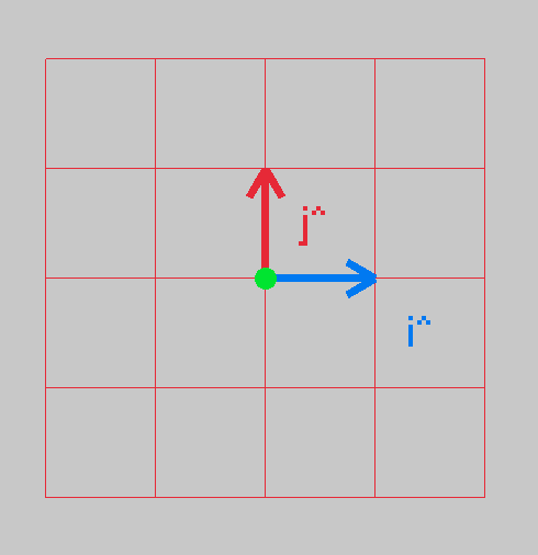
These two basis vectors, which are actually the columns of a 2D transformation matrix, define your space:
\[\text{2D transformation matrix} = \begin{bmatrix} a & b \\ c & d \\ \end{bmatrix}\]This is a typical 2D transformation matrix, you take your input (\(x\) and \(y\)) and multiple by this, to get your new point. But, what’s fascinating, is that the columns are the \(\hat{i}\) and \(\hat{j}\)! EG, let’s look at our example above. Let’s take the point \((1,0)\) and see where it lands.
\[A = \begin{bmatrix} 1 & 0 \\ 0 & 1 \\ \end{bmatrix} \cdot \begin{bmatrix} 1 \\ 0 \\ \end{bmatrix} = \begin{bmatrix} (1 \cdot 1) + (0 \cdot 0) \\ (0 \cdot 1) + (1 \cdot 0) \\ \end{bmatrix} = \begin{bmatrix} 0 + 1 \\ 0 + 0 \\ \end{bmatrix} = \begin{bmatrix} 1 \\ 0 \\ \end{bmatrix} = \hat{i}\]So, we can see, that we’ve just extracted the \(\hat{i}\) term.
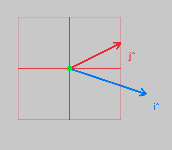
When we have a new 2D transform, say, \(B = \begin{bmatrix} 3 & 2 \\ 1 & 1 \\ \end{bmatrix}\)
These are now the new basis vectors. We can apply this 2D transform to all grid lines, and see how the space is warped.
First, let’s look at the new basis vectors, how they look:
And now, let’s transform the grid lines to see how the fabric of space changes:
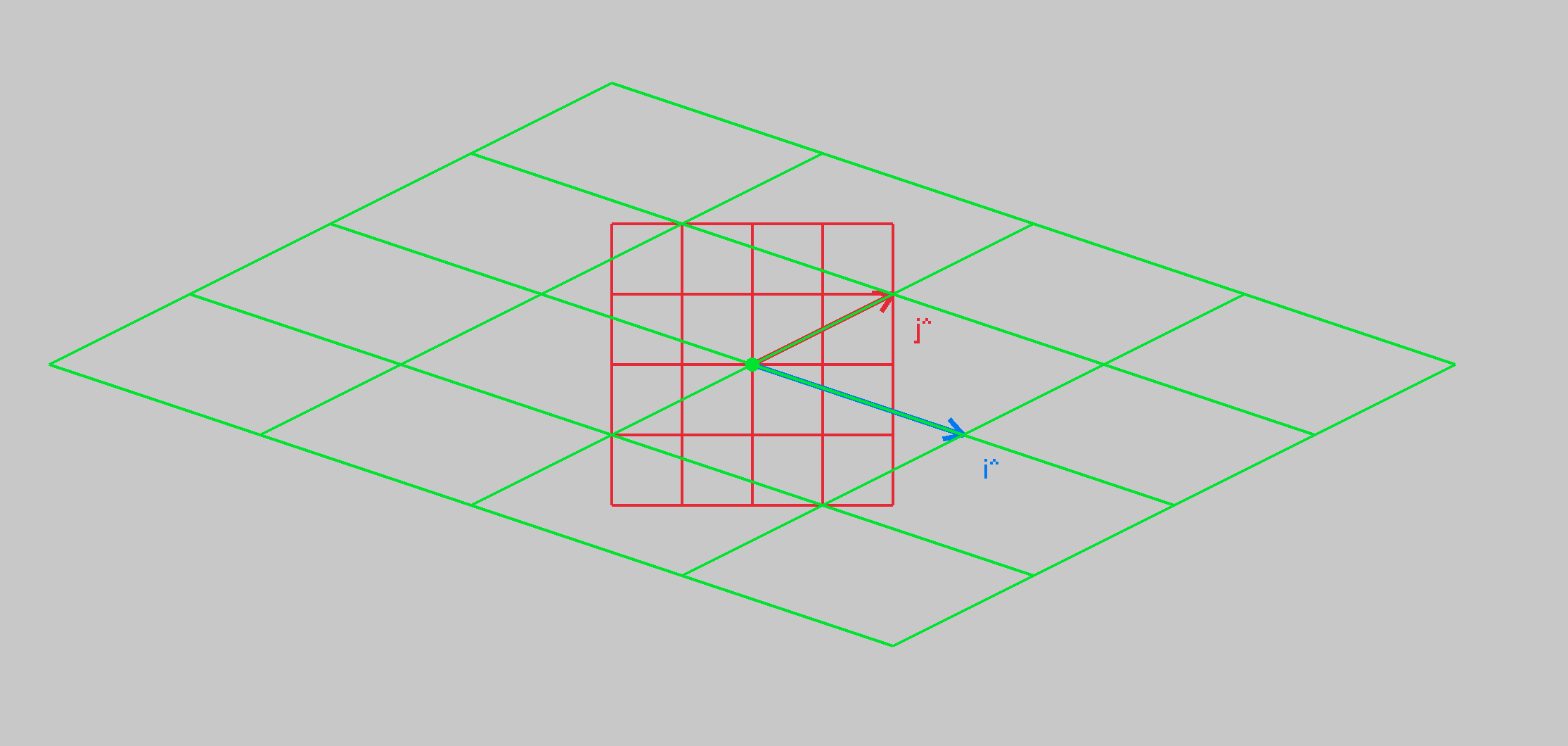
As we can see, the grid space now lines up with the new basis vectors, pretty cool!
Next, before we go back to linear regression (this has taken a major tangent), i’ll animate the change of grid lines, 3b1b style!
04/04/2026
And there we have it, if we interpolate between the identity matrix, and our target transform. The enabler is the LERP or LinEar inteRPolation. Basically, how we transition, in discrete steps, from one thing to another.
\[\text{LERP} = start \cdot \lambda \cdot (\text{end} - \text{start})\]\(\lambda\) in this case, is some scaler, if we use \(\lambda \in \[ 0, 1\]\) then we can take a percentage of the target and add it to the start. If \(\lambda\) is scale nicely from 0 -> 1 -> 0 then we can nicely LERP between our start (identity matrix) and target, our desired final transform. We than have a slightly warped transform, which we can now use to warp our grid lines by. We do this over and over, and we get the view from above!
24/05/26
Been a while since I worked on this - focusing on some other projects, but I’d like to get this to at least a state where I no longer have to protect some random pieces of paper that I’ve had on my desk for ages, with my notes on what I was working on. Mostly, it was on a quick derivation of a rotation matrix, that generalises the rotation some more.
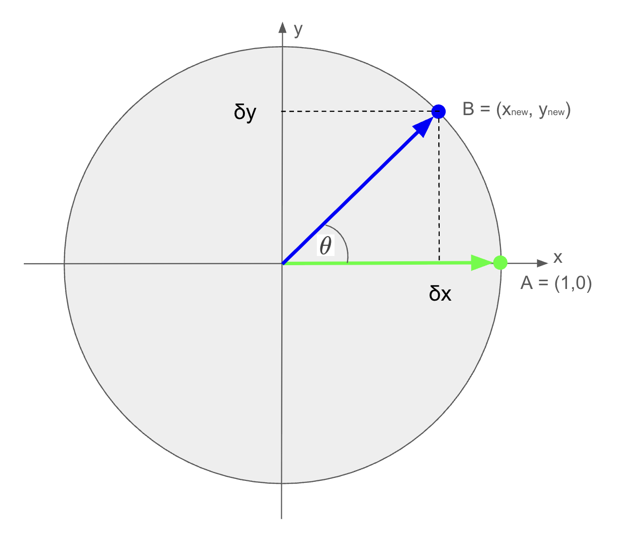
What we want is a 2D matrix that transforms a point to a new basis, \(\hat{i_{new_{x}}} \text{ and } \hat{j_{new_{x}}}\), and it’s y counterpart - \(\hat{i_{new_{y}}} \text{ and } \hat{j_{new_{y}}}\)
That is:
\[\begin{bmatrix} x_{new} \\ y_{new} \\ \end{bmatrix} = \begin{bmatrix} \hat{i_{new_{x}}} && \hat{i_{new_{y}}} \\ \hat{j_{new_{x}}} && \hat{j_{new_{y}}} \\ \end{bmatrix} \cdot \begin{bmatrix} x \\ y \\ \end{bmatrix}\]Let’s take a look at the unit circle: